An ocean from a wave spectrum

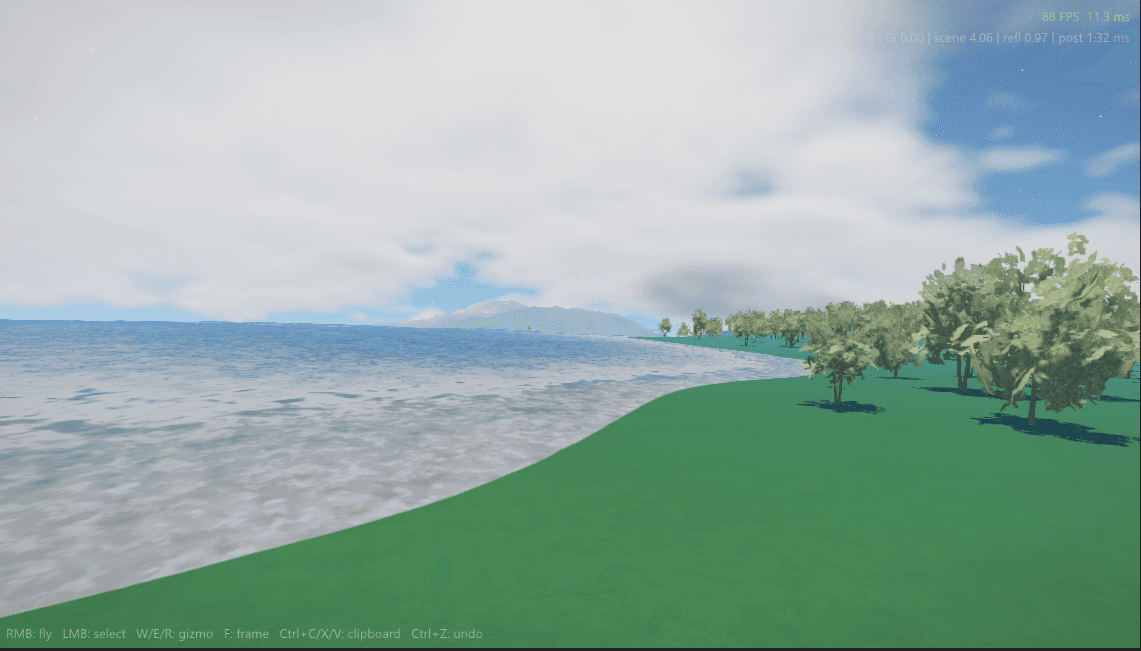
You cannot keyframe an ocean. What you can do is steal sixty years of oceanography: measure how wave energy distributes across wavelengths, synthesize a surface with that exact statistical fingerprint, and let an inverse FFT animate it. This is how film water has worked since Titanic, and it is how REACT's oceans work in real time.

11 min
5 figures
Updated June 2026

256 x 256

FFT grid

cascades

1,000 m

largest patch

1.6 ms

total cost

Waves are a statistics problem

Watch open water for a minute and you will see that it is not one wave but a crowd of them: long swells rolling under short chop, all moving at different speeds. Oceanographers describe this crowd with an energy spectrum, a curve that says how much wave energy lives at each wavelength for a given wind. REACT uses the Phillips spectrum, the classic choice for graphics:

Eq 01

Auto-touring terms

\htmlClass{eq-hl-0}{P(k)} \;=\; A\,\frac{\exp\!\left(-1/(k\htmlClass{eq-hl-1}{L})^{2}\right)}{k^{4}}, \qquad \htmlClass{eq-hl-1}{L} = \frac{\htmlClass{eq-hl-2}{V^{2}}}{\htmlClass{eq-hl-3}{g}}

each symbol, explained —

Energy falls off steeply at short wavelengths (the k to the fourth in the denominator) and is cut off entirely for waves longer than the wind can build (the exponential).

Fig. 1

5 m/s breeze

10 m/s fresh wind

15 m/s near gale

The Phillips spectrum for three wind speeds, on a log energy scale. Stronger wind does two things at once: it shifts the peak toward longer waves, and it raises total energy by orders of magnitude. A 15 m/s sea is not a scaled-up 5 m/s sea, and the simulation reflects that.

From spectrum to moving surface

The spectrum tells you how big each wave component is. To get an actual surface, REACT fills a 256 by 256 grid of frequencies with random amplitudes drawn from the spectrum, then advances each one in time using the deep water dispersion relation, which says longer waves travel faster. An inverse fast Fourier transform collapses all of them into a heightfield in one shot:

Eq 02

Auto-touring terms

\htmlClass{eq-hl-0}{h(\mathbf{x}, t)} \;=\; \sum_{\mathbf{k}} \htmlClass{eq-hl-1}{\tilde{h}(\mathbf{k}, t)}\; e^{\,i\,\htmlClass{eq-hl-2}{\mathbf{k}}\cdot\mathbf{x}}

each symbol, explained —

The surface height is the sum of every frequency component. Computed naively this is millions of sine evaluations; as an inverse FFT it is a few dozen GPU microseconds.

Two refinements matter visually. First, the same spectral data yields horizontal displacement, which sharpens wave crests from rolling sine waves into proper peaked seas. Second, where that displacement compresses the surface past folding, the math flags it, and that flag is exactly where breaking foam belongs. Foam in REACT is not painted on; it is the simulation confessing that a wave just broke.

Near shore, a second rule takes over: McCowan's depth-limited breaking criterion, which says a wave breaks when its height reaches roughly 0.78 of the water depth. That single ratio is why surf lines up along the coast in REACT instead of breaking at random. Out at sea, total whitecap coverage is calibrated against Monahan and O'Muircheartaigh's wind-speed power law, and in strong winds the foam organizes into the long streaks aligned with the wind that Langmuir circulation produces on real oceans.

shaders/ocean_evolve.comp (simplified)

// advance one frequency component to time t
float k     = length(waveVector);
float omega = sqrt(9.81 * k);            // deep water dispersion:
                                         // longer waves travel faster
vec2 phase  = vec2(cos(omega * t), sin(omega * t));

// pairing each component with its conjugate keeps height real-valued
htilde[id]  = ComplexMul(h0[id],  phase)
            + ComplexMul(h0Conj[id], vec2(phase.x, -phase.y));

That dispersion relation deserves its own figure, because it is the single biggest reason FFT water reads as ocean rather than jelly. Every wavelength moves at its own speed, so the surface continuously decorrelates: chop flickers, swell rolls, and the two visibly slide past each other exactly as they do at sea.

Fig. 2

phase speed c = sqrt(g lambda / 2 pi)

Deep water phase speed against wavelength. A 2 m chop wave crawls at walking pace while a 200 m swell moves at storm-chase speed; because the FFT advances every component by this exact curve, the relative motion is physically correct at all scales simultaneously.

Fig. 3

Spectrum init

Fill the frequency grid from the Phillips spectrum for the current wind. Runs only when weather changes.

Time evolution

Advance each component by the dispersion relation: longer waves travel faster.

Inverse FFT

Collapse the spectrum into height and horizontal displacement maps.

Derive maps

Normals from gradients, foam from the folding test, all in the same pass.

Shade

Three cascades blended by distance, lit with absorption, subsurface and sky reflection.

The per-frame ocean pipeline. Everything through the FFT runs in compute shaders; the three cascades use the same code at three world scales.

A single 256-cell patch would tile visibly across a planet, so REACT runs three cascades of the same simulation at patch sizes of 25, 160 and 1,000 meters and sums them. Each point on the ocean gets detail from all three, and the repeat distance grows to kilometers, far beyond what the eye picks up. The whole stack costs around 0.9 ms of simulation plus 0.7 ms of shading.

Cascade	Patch size	Carries wavelengths	Visual role
0 (detail)	25 m	0.2 to 12 m	ripples and chop, the sparkle under direct sun
1 (sea state)	160 m	12 to 80 m	the waves you would actually surf
2 (swell)	1,000 m	80 to 500 m	long rolling energy from distant weather

Tip

Changing the wind re-seeds the spectrum, which would make the whole ocean snap to a new state. REACT cross-fades between the old and new spectra over two seconds, so weather changes roll in instead of teleporting.

Fig. 4

128 x 128visible tiling0.0 ms

256 x 256REACT, per cascade0.0 ms

512 x 512film-style detail0.0 ms

1024 x 1024offline territory0.0 ms

Cost of one simulation cascade per frame at different grid resolutions, measured on the reference RTX 4070. Three 256-cell cascades beat one 512-cell grid on both quality and cost, which is why cascades win.

Why deep water looks dangerous

The surface is half the ocean. The other half is what happens to light underneath it, and it is governed by the same Beer-Lambert law the atmosphere article used, with very different constants. Water absorbs red light about thirteen times faster than blue. Ten meters down, red is effectively gone; by sixty meters even green is fading and the world is monochrome blue.

Fig. 5

red (k = 0.45 / m)

green (k = 0.065 / m)

blue (k = 0.035 / m)

Sunlight surviving to depth in clear ocean water, per color channel. REACT evaluates these exact exponentials in the water shader, which is why shallows read warm and inviting while depth reads cold without a single hand-tuned color grade.

Two details of the surface lighting come straight from oceanography as well. The band of sun glitter stretching toward the horizon follows Cox and Munk's 1954 slope statistics, originally measured from aerial photographs of the Pacific: wind roughens the surface, the slope distribution widens, and the glitter band spreads exactly as their data says it should. And the absorption constants plotted above are Jerlov's type I clear ocean water; his murkier coastal types are the dial REACT will turn for harbors and river mouths.

Everything else in the water column follows from this curve plus the systems already described: caustics are the wave normals focusing sunlight, light shafts are the atmosphere's volumetric scattering reused underwater, and buoyancy comes from sampling the displaced heightfield, so boats ride the same waves you see. One simulation, observed from both sides of the surface.

Known issue

Buoyancy samples the heightfield at the hull's position from the previous frame, so an object teleported onto water can take one frame to find the surface. Harmless in play, visible in editor stress tests.

Console variables

The ocean reads its configuration from the console like every other system:

Variable	Default	Description
o_fft_size	256	Frequency grid resolution per cascade. See Fig. 4 for the cost curve before raising it.
o_cascades	3	Simulation cascades at 25, 160 and 1,000 m patch sizes, summed at every point.
o_wind_speed	10	Wind speed in m/s feeding the Phillips spectrum. Usually driven by the weather system, can be forced for testing.
o_choppiness	1.4	Scale on horizontal displacement. Zero gives rolling sine swells; past 1.8 crests start to self-intersect.
o_foam_decay	0.92	Per-second retention of foam after the folding test triggers it. Lower clears whitecaps faster.
o_absorption_rgb	0.45 0.065 0.035	Beer-Lambert absorption per channel per meter, the exact constants plotted in Fig. 5.

An ocean from a wave spectrum

Waves are a statistics problem

From spectrum to moving surface

Spectrum init

Time evolution

Inverse FFT

Derive maps

Shade

Why deep water looks dangerous

Console variables

Further reading

An ocean from a wave spectrum

Waves are a statistics problem

From spectrum to moving surface

Spectrum init

Time evolution

Inverse FFT

Derive maps

Shade

Why deep water looks dangerous

Console variables

Further reading